3일차(데이터 가공)
#csv파일과 tsv파일의 차이점
| csv(Comma-separated values) | 데이터를 , (콤마) 로 구분 |
| tsv(Tab-separated values) | 데이터를 \n (탭)으로 구분 |
#pandas를 이용하여 csv파일 불러오기
import pandas as pd
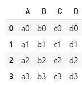
df=pd.read_csv('concat_1.csv',sep=',')
df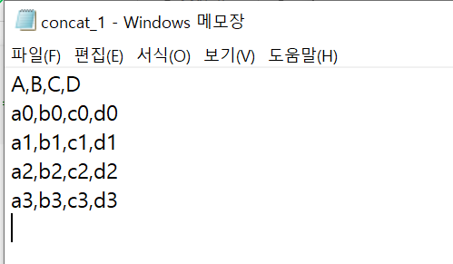
#pandas로 tsv 파일 불러오기
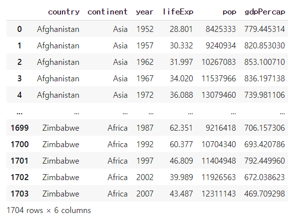
df=pd.read_csv('gapminder.tsv',sep='\t')
df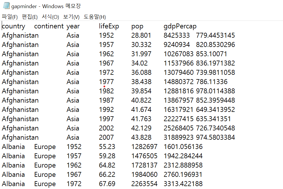
#head() 함수
df.head() #첫 다섯 줄 불러옴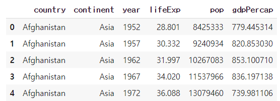
# tail함수
df.tail() #마지막 다섯줄 불러옴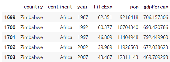
#columns 함수
>df.columns     #컬럼명 출력

Index(['country', 'continent', 'year', 'lifeExp', 'pop', 'gdpPercap'], dtype='object')
#info() 함수
>df.info()   # 데이터의 전체적인 정보 조회

<class 'pandas.core.frame.DataFrame'>
RangeIndex: 1704 entries, 0 to 1703
Data columns (total 6 columns):
 #   Column     Non-Null Count  Dtype
---  ------     --------------  -----
 0   country    1704 non-null   object
 1   continent  1704 non-null   object
 2   year       1704 non-null   int64
 3   lifeExp    1704 non-null   float64
 4   pop        1704 non-null   int64
 5   gdpPercap  1704 non-null   float64
dtypes: float64(2), int64(2), object(2)
memory usage: 80.0+ KB
##pandas에서 object 란 문자열을 의미
#dtypes함수
>df.dtypes     #데이터 타입 조회

country       object
continent     object
year           int64
lifeExp      float64
pop            int64
gdpPercap    float64
dtype: object
#한가지 열에만 접근하기
>df['country'] #country열에만 접근

0       Afghanistan
1       Afghanistan
2       Afghanistan
3       Afghanistan
4       Afghanistan
           ...
1699       Zimbabwe
1700       Zimbabwe
1701       Zimbabwe
1702       Zimbabwe
1703       Zimbabwe
Name: country, Length: 1704, dtype: object
#여러열에 접근하기
df[{'country','continent','year'}]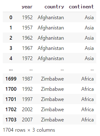
#행에 접근하기
>df.loc[0]          #행이름이 0인 것에 접근


country      Afghanistan
continent           Asia
year                1952
lifeExp           28.801
pop              8425333
gdpPercap        779.445
Name: 0, dtype: object
>df.iloc[0]       #위치로 접근=0번째에 접근


country      Afghanistan
continent           Asia
year                1952
lifeExp           28.801
pop              8425333
gdpPercap        779.445
Name: 0, dtype: object| loc | 행 이름 기준으로 접근 |
| iloc | 행 위치 기준으로 접근 |
df.loc[[0,10,100,1000]]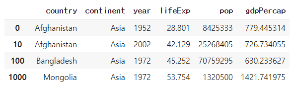
#행/열 접근하기
df.loc[[0,10,100,1000],['year','country']] #0,10,100,1000행에 대해 year,country열 접근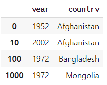
df.iloc[[0,10,100,1000],[0,2]]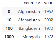
df.loc[:,['year','country']] #모든 행에 대해 year,country열 접근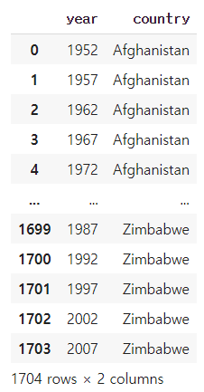
#groupby()함수
df #df 변수에 저장된 concat_1.csv 파일 조회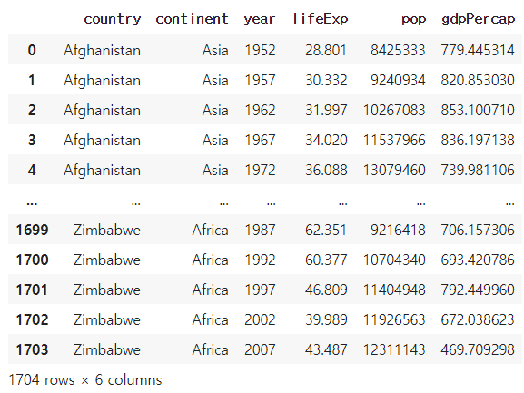
>a=df.groupby('year')['lifeExp'].mean()   #같은 생년월일끼리 모아 기대수명 평균내기
>a

year
1952    49.057620
1957    51.507401
1962    53.609249
1967    55.678290
1972    57.647386
1977    59.570157
1982    61.533197
1987    63.212613
1992    64.160338
1997    65.014676
2002    65.694923
2007    67.007423
Name: lifeExp, dtype: float64
##a라는 변수에 year열을 기준으로 lifeExp의 평균값을 출력
##mean() 함수는 평균 값을 구함.
#엑셀 저장 함수
a.to_excel('result.xlsx') #result 라는 이름으로 엑셀에 저장
#plot 함수
a.plot() #그래프 그려주는 함수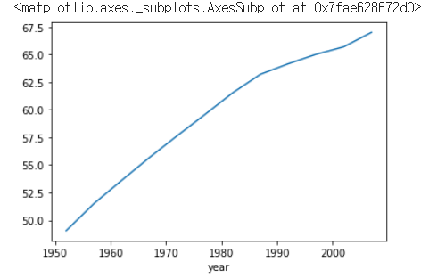
#같은 연도생 안에서 같은 대륙별로 기대수명의 평균내기
>a=df.groupby(['year','continent'])['lifeExp'].mean()
>a


year  continent
1952  Africa       39.135500
      Americas     53.279840
      Asia         46.314394
      Europe       64.408500
      Oceania      69.255000
1957  Africa       41.266346
      Americas     55.960280
      Asia         49.318544
      Europe       66.703067
      Oceania      70.295000
...........생략..............
2002  Africa       53.325231
      Americas     72.422040
      Asia         69.233879
      Europe       76.700600
      Oceania      79.740000
2007  Africa       54.806038
      Americas     73.608120
      Asia         70.728485
      Europe       77.648600
      Oceania      80.719500
Name: lifeExp, dtype: float64
#count()함수
>df.groupby('continent')['country'].count()         #대륙별 사람 숫자

continent
Africa      624
Americas    300
Asia        396
Europe      360
Oceania      24
Name: country, dtype: int64
#nunique() 함수
>df.groupby('continent')['country'].nunique()

continent
Africa      52
Americas    25
Asia        33
Europe      30
Oceania      2
Name: country, dtype: int64
##nunique 함수는 중복되는 데이터는 제거한 후의 수를 나타냄.
##대륙별로 접근하여 나라가 몇개 있는지 출력
#열(Series) 생성하기
>a=pd.Series([100,150,200,250,300])     #새로운 열 만들기
>a

0    100
1    150
2    200
3    250
4    300
dtype: int64
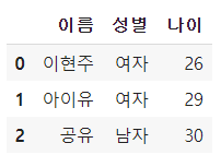
#여러열 만들기
pd.DataFrame({

      '이름':['이현주','아이유','공유'],
      '성별':['여자','여자','남자'],
      '나이':['26','29','30']

})
#describe()함수
df.describe()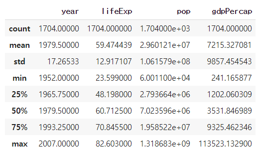
##describe 함수는 데이터의 평균, 표준편차,중간값, 최대,최소 등 통계값들을 보여줌.
#info() 함수
scientists=pd.read_csv("scientists.csv")  #scientists라는 변수에 파일 저장
scientists                                # 파일 조회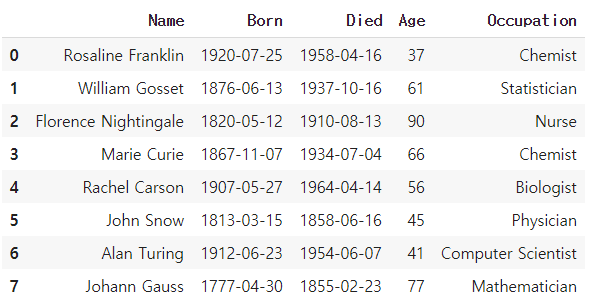
>scientists.info()


<class 'pandas.core.frame.DataFrame'>
RangeIndex: 8 entries, 0 to 7
Data columns (total 5 columns):
 #   Column      Non-Null Count  Dtype
---  ------      --------------  -----
 0   Name        8 non-null      object
 1   Born        8 non-null      object
 2   Died        8 non-null      object
 3   Age         8 non-null      int64
 4   Occupation  8 non-null      object
dtypes: int64(1), object(4)
memory usage: 448.0+ bytes
>>>이상한 점! Born데이터와 Died 데이터가 숫자임에도 불구하고 데이터타입이 object(문자열)로 나온다는 점!
왜일까?? 그 이유는 숫자들 사이에 '-' 때문에 데이터를 문자열로 인식!
#문자열로 인식되는 숫자데이터를 컴퓨터가 숫자로 인식할 수 있게 바꿔주기
born_dt=pd.to_datetime(scientists['Born'],format='%Y-%m-%d') #format함수로 형태를 알려줘야함
died_dt=pd.to_datetime(scientists['Died'],format='%Y-%m-%d')

scientists['Born']=born_dt
scientists['Died']=died_dt
scientists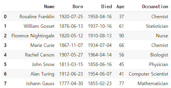
>scientists.info()       #데이터 타입이 바뀌었는지 확인하기


<class 'pandas.core.frame.DataFrame'>
RangeIndex: 8 entries, 0 to 7
Data columns (total 5 columns):
 #   Column      Non-Null Count  Dtype
---  ------      --------------  -----
 0   Name        8 non-null      object
 1   Born        8 non-null      datetime64[ns]
 2   Died        8 non-null      datetime64[ns]
 3   Age         8 non-null      int64
 4   Occupation  8 non-null      object
dtypes: datetime64[ns](2), int64(1), object(2)
memory usage: 448.0+ bytes
##object 였던 데이터타입이 datetime64 로 바뀜.
scientists['Days']=scientists['Died']-scientists['Born']   #Days 라는 새로운 열 만들어 Died-Born데이터 값 저장
scientists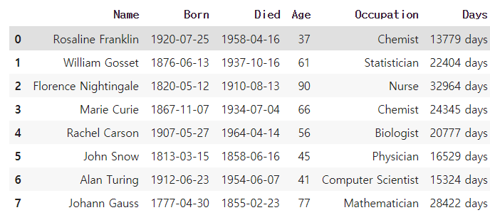
#여러 통계값을 구하는 함수들
>age=scientists['Age']     #age 라는 변수에 scientitsts 변수에 저장되어 있는 데이터 중 Age열의 데이터만 저장
>age

0    37
1    61
2    90
3    66
4    56
5    45
6    41
7    77
Name: Age, dtype: int64


>age.mean()
59.125

>age.max()
90

>age.min()
37

>age.median()
58.5
#함수들 이용하여 원하는 데이터 접근하기
>age[age>age.mean()]     #age의 평균값보다 큰 age 값만 뽑기

1    61
2    90
3    66
7    77
Name: Age, dtype: int64


>age>age.mean() #true 값만 출려하는 것..

0    False
1     True
2     True
3     True
4    False
5    False
6    False
7     True
Name: Age, dtype: bool
scientists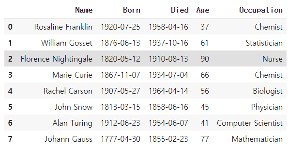
scientists[age>age.mean()]     #age의 값이 age의 평균값보다 큰 행을 가져오기

scientists[scientists['Age']>scientists['Age'].mean()]    #위와 같은 값을 출력함.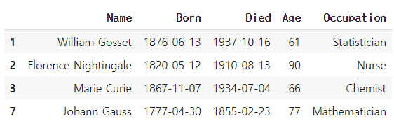
#열의 개수가 같은 열끼리의 덧셈
>age+age    #(열의 개수가 같을 때)열끼리의 덧셈 가능

0     74
1    122
2    180
3    132
4    112
5     90
6     82
7    154
Name: Age, dtype: int64
#열에 수 더하기
>age+100

0    137
1    161
2    190
3    166
4    156
5    145
6    141
7    177
Name: Age, dtype: int64
#열의 개수가 다른 열끼리의 덧셈
>a=pd.Series([100,100]) #2개의 열 생성
>a

0    100
1    100
dtype: int64


>age+a #2개의 열과 8개의 열을 더하기

0    137.0
1    161.0
2      NaN
3      NaN
4      NaN
5      NaN
6      NaN
7      NaN
dtype: float64